The OpenAQ API has the ability to perform geospatial queries,
enabling you to retrieve data based on location. This vignette will
guide you through the two primary geospatial query methods available in
openaq: point and radius searches, and bounding box
searches.
openaq provides access to two methods for querying
locations on the OpenAQ platform geospatially:
Point and Radius: Searches around a given point coordinate (latitude, longitude) at a specified radius in meters. This is ideal for finding air quality data within a certain distance of a specific location.
Bounding Box: Searches within a spatial bounding box defined as a list of four coordinates:
xmin,ymin,xmax, andymax. This method is useful for querying data within a rectangular area.
Point and Radius
The list_location() function allows you to search for
locations near a given point. You provide the latitude and longitude of
the center point, as well as the radius within which to search. The
radius is specified in meters, with a maximum value of 25,000 (25
kilometers).
locs <- list_locations(
  coordinates = c(latitude = -36.7724, longitude = -73.0666), # the coordinates in Concepción, Chile.
  radius = 25000 # 10,000 meters or 10 kilometers
)
head(locs)
#>    id              name is_mobile is_monitor         timezone countries_id
#> 1  26           Inpesca     FALSE       TRUE America/Santiago            3
#> 2  65          Punteras     FALSE       TRUE America/Santiago            3
#> 3  69  Kingston College     FALSE       TRUE America/Santiago            3
#> 4 210 Liceo Polivalente     FALSE       TRUE America/Santiago            3
#> 5 356          Bocatoma     FALSE       TRUE America/Santiago            3
#> 6 808            Indura     FALSE       TRUE America/Santiago            3
#>   country_name country_iso  latitude longitude      datetime_first
#> 1        Chile          CL -36.73720 -73.10443 2016-01-30 01:00:00
#> 2        Chile          CL -36.92333 -73.03613 2016-01-30 01:00:00
#> 3        Chile          CL -36.78465 -73.05206 2016-01-30 01:00:00
#> 4        Chile          CL -36.60171 -72.95852 2016-02-01 17:00:00
#> 5        Chile          CL -36.80303 -73.12053 2016-05-10 20:00:00
#> 6        Chile          CL -36.76980 -73.11371 2016-01-30 01:00:00
#>         datetime_last                        owner_name providers_id
#> 1 2026-03-09 18:00:00 Unknown Governmental Organization          164
#> 2 2026-03-09 18:00:00 Unknown Governmental Organization          164
#> 3 2026-03-09 18:00:00 Unknown Governmental Organization          164
#> 4 2026-03-09 18:00:00 Unknown Governmental Organization          164
#> 5 2026-03-09 18:00:00 Unknown Governmental Organization          164
#> 6 2026-03-09 18:00:00 Unknown Governmental Organization          164
#>   provider_name
#> 1 Chile - SINCA
#> 2 Chile - SINCA
#> 3 Chile - SINCA
#> 4 Chile - SINCA
#> 5 Chile - SINCA
#> 6 Chile - SINCA
In this example, we are searching for locations within a 10 kilometer radius of the specified latitude and longitude. The result will be a list of locations that fall within this circular area.
Bounding box
For queries covering a rectangular area, you can use the
list_locations() function with the bbox argument. You need
to provide the minimum and maximum longitude (xmin,
xmax) and latitude (ymin, ymax)
values that define the corners of your bounding box.
locs <- list_locations(
  bbox = c(
    xmin = -8.478184,
    ymin = 26.640174,
    xmax = 50.803066,
    ymax = 46.534067
  )
)
head(locs)
#>    id                         name is_mobile is_monitor        timezone
#> 1  34 SPARTAN - Weizmann Institute     FALSE       TRUE  Asia/Jerusalem
#> 2 420                    Vijećnica     FALSE       TRUE Europe/Sarajevo
#> 3 421                        Otoka     FALSE       TRUE Europe/Sarajevo
#> 4 422                       Tetovo     FALSE       TRUE Europe/Sarajevo
#> 5 423                   Ivan Sedlo     FALSE       TRUE Europe/Sarajevo
#> 6 584                      Harmani     FALSE       TRUE Europe/Sarajevo
#>   countries_id           country_name country_iso latitude longitude
#> 1           11                 Israel          IL   31.907    34.810
#> 2          132 Bosnia and Herzegovina          BA   43.859    18.435
#> 3          132 Bosnia and Herzegovina          BA   43.848    18.364
#> 4          132 Bosnia and Herzegovina          BA   44.290    17.895
#> 5          132 Bosnia and Herzegovina          BA   43.715    18.036
#> 6          132 Bosnia and Herzegovina          BA   44.916    17.349
#>   datetime_first datetime_last                        owner_name providers_id
#> 1             NA            NA Unknown Governmental Organization          226
#> 2     1464771600    1539464400 Unknown Governmental Organization          159
#> 3     1461708000    1539464400 Unknown Governmental Organization          159
#> 4     1461708000    1539464400 Unknown Governmental Organization          159
#> 5     1461708000    1539464400 Unknown Governmental Organization          159
#> 6     1465815600    1470556800 Unknown Governmental Organization          159
#>   provider_name
#> 1       Spartan
#> 2        Bosnia
#> 3        Bosnia
#> 4        Bosnia
#> 5        Bosnia
#> 6        Bosnia
This query will return all locations within the defined rectangular region.
bbox_coords <- c(-8.478184, 26.640174, 50.803066, 46.534067)
names(bbox_coords) <- c("xmin", "ymin", "xmax", "ymax")
bbox <- st_as_sfc(st_bbox(bbox_coords), crs = 4326)
world_sp <- maps::map("world", plot = FALSE, fill = TRUE)
world_sf <- st_as_sf(world_sp)
plot(st_geometry(world_sf), col = "lightgray", border = "black", xlim = st_bbox(bbox)[c("xmin", "xmax")], ylim = st_bbox(bbox)[c("ymin", "ymax")])
plot(st_geometry(bbox), lwd = 2, add = TRUE)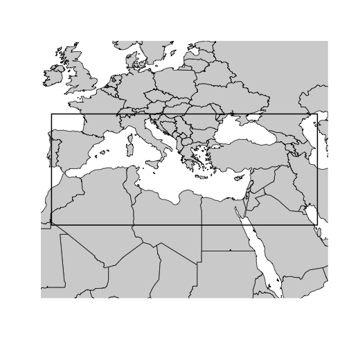
Computing a bounding box from a polygon
Often, you’ll want to query data within a specific geographic area defined by a polygon, rather than a simple rectangle. Real-world boundaries are often complex shapes. For instance, consider the boundary of the city of Los Angeles, which has a complex, irregular shape.
url <- "https://maps.lacity.org/lahub/rest/services/Boundaries/MapServer/7/query?outFields=*&where=1%3D1&f=geojson"
la <- sf::st_read(url)
plot(la["OBJECTID"])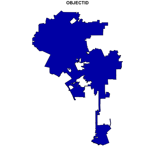
We can use the sf package to read the GeoJSON data
representing the city boundary.
To derive a bounding box from this polygon, we can use the
sf::st_bbox() method. This function calculates the minimum
and maximum x and y coordinates of the polygon, effectively creating a
bounding box that encompasses the entire shape. The output is a named
numeric vector, perfectly formatted for the bbox parameter in the
openaq function.
bbox <- sf::st_bbox(la)
bbox
#>       xmin       ymin       xmax       ymax
#> -118.66819   33.70366 -118.15537   34.33731
This output gives you the xmin, ymin, xmax, and ymax values needed
for your openaq query.
bbox <- sf::st_bbox(la)
world_sp <- maps::map("county", plot = FALSE, fill = TRUE)
world_sf <- st_as_sf(world_sp)
plot(
  st_geometry(world_sf),
  col = "lightgray",
  border = "black",
  xlim = st_bbox(bbox)[c("xmin", "xmax")],
  ylim = st_bbox(bbox)[c("ymin", "ymax")]
)
plot(sf::st_as_sfc(bbox), lwd = 2, lty = 2, add = TRUE)
plot(st_geometry(la), lwd = 2, add = TRUE)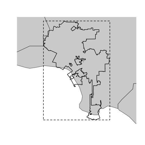
This map shows the Los Angeles city boundary along with the calculated bounding box.
locations <- list_locations(
  bbox = bbox
)
plot(
  st_geometry(world_sf),
  col = "lightgray",
  border = "black",
  xlim = st_bbox(bbox)[c("xmin", "xmax")],
  ylim = st_bbox(bbox)[c("ymin", "ymax")]
)
plot(st_geometry(la), lwd = 2, add = TRUE)
plot(sf::st_as_sfc(bbox), lwd = 2, lty = 2, add = TRUE)
points(locations$longitude, locations$latitude, col = "#6a5cd8", pch = 15)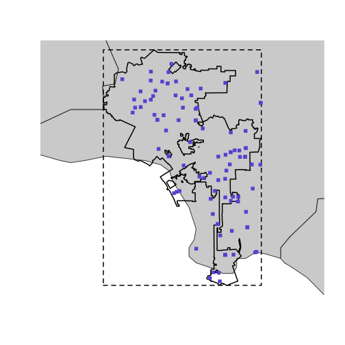
Now, you can directly use the bbox object generated by
sf::st_bbox() in your list_locations() call.
This will retrieve air quality data within the bounding box that
encompasses the city of Los Angeles.
For a detailed explanation about how the OpenAQ API works with these methods, see the official OpenAQ API documentation at https://docs.openaq.org/using-the-api/geospatial. This documentation provides further information on the available parameters and how to optimize your geospatial queries.