querying-measurements

library(openaq)

Introduction

This vignette demonstrates how to use the openaq R package to query air quality measurements from the OpenAQ API. We will walk through the process of retrieving a list of locations, inspecting their sensors and parameters, and finally, fetching and plotting the actual measurements for a specific sensor.

Listing Locations

The list_locations() function allows us to retrieve information about monitoring locations. We can filter locations based on parameters and countries. Here, we are searching for locations that measure PM_2.5 (parameter ID 2) in Madagascar (country ID 182). By default resource functions return a data frame but we set as_data_frame = FALSE to receive the data as a list, which we will use for easier inspection in the following steps.

locations <- list_locations(
  parameters_id = 2,
  countries_id = 182,
  as_data_frame = FALSE
)

The locations object is a list, where each element represents a monitoring location. Let’s examine the first location in the list and explore its sensors.

location <- locations[[1]]
sensors <- location$sensors
sensors
# > [[1]]
# > [[1]]$id
# > [1] 225221
# >
# > [[1]]$name
# > [1] "pm25 µg/m³"
# >
# > [[1]]$parameter
# > [[1]]$parameter$id
# > [1] 2
# >
# > [[1]]$parameter$name
# > [1] "pm25"
# >
# > [[1]]$parameter$units
# > [1] "µg/m³"
# >
# > [[1]]$parameter$displayName
# > [1] "PM2.5"

Each location contains information about its sensors. Each sensor has an id, name, and details about the measured parameter, including its name, units, and ID.

Each location also provides the timezone of where it is local, which will be helpful when querying measurements, so we will store this for later.

tz <- location$timezone
tz
# > [1] "Indian/Antananarivo"

To fetch measurements, we need the sensor ID. This location only measures PM_2.5 and in turn only has one sensor so we can extract it as follows:

sensors_id <- sensors[[1]]$id
sensors_id
# > [1] 225221

Fetching Measurements

Now we can use the list_sensor_measurements() function to retrieve the measurements for the sensor. We need to provide the sensors_id, datetime_from, and datetime_to arguments. We will query for all measurements during the month of January 2025.It is important to use the correct timezone for your dates, we use the timezone for location that we stored in the tz variable above. The limit argument controls the maximum number of measurements returned in a single page of results. Because this is hourly data, and we are querying 31 days of measurements, we will be able to view all the results in one page (24 hourly measurements * 31 days = 744 measurements).

measurements <- list_sensor_measurements(
  sensors_id,
  datetime_from = as.POSIXct("2025-01-01", tz = tz),
  datetime_to = as.POSIXct("2025-01-31", tz = tz),
  limit = 1000
)

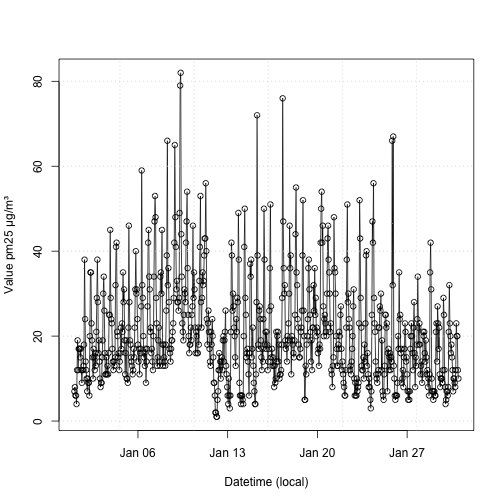
Finally, we can visualize the measurements using the plot() function.

plot(measurements)