The OpenAQ API has the ability to provide measurement in the original
reported time period as well as aggregated to larger time periods.
openaq provides methods to access these various periods of
data, and includes additional descriptive statistics and coverage
information.
Many public health standards rely on daily or yearly means so having access to these values precomputed allows for easier access and comparison. The World Health Organization (WHO) sets the daily PM2.5 guideline to 15 µg/m³.
This vignette will demonstrate how to query data using
openaq and get results to compare against public health
benchmarks like the WHO daily PM2.5 standard.
set_api_key("replace-me-with-a-valid-openaq-api-key")The list_sensor_measurements() function provides
precomputed aggregations through the data argument. This argument
defaults to measurements or the original measurement
period. The full list of options includes: measurements,
hours, days, years. As an example
we will query PM2.5 data from sensor 3646869,
from the ‘Mari - Industrial Station’ location in the Republic of Cyprus.
To compare against the WHO daily guideline, we will request data
aggregated to the day, using the days option:
data <- list_sensor_measurements(
  3646869,
  data = "days",
  datetime_from = as.POSIXct("2025-01-01", tz = "Asia/Nicosia"),
  datetime_to = as.POSIXct("2025-05-31", tz = "Asia/Nicosia"),
  limit = 1000
)
The measurements resource provides coverage information when
aggregating data into time periods. This helps provide transparency into
the data coverage and help us decide if the resulting mean is
representative. This completeness is computed based on the result of
dividing observed_count by expected_count, in
the case of a days average and hourly measurement, we
expect 24 measurements to be the complete period.
head(data[, c("value", "percent_complete", "expected_count", "observed_count")])
#>   value percent_complete expected_count observed_count
#> 1  19.0              100             24             24
#> 2  18.5              100             24             24
#> 3  18.4              100             24             24
#> 4  17.2              100             24             24
#> 5  27.7              100             24             24
#> 6  20.0              100             24             24
We can filter out values by accessing the
percent_complete field. A commonly used threshold for data
completeness is 75%, in the case of a daily average at least 18 out of
24 hours.
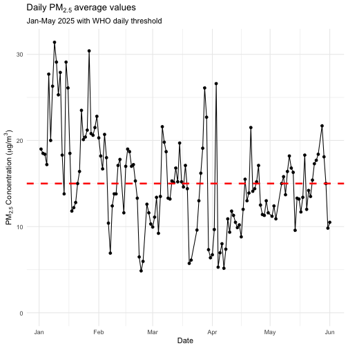
data <- data[data$percent_complete > 75, ]We can now plot the daily average time series and compare it against
the WHO daily threshold value with ggplot2:
ggplot(data, aes(x = as.Date(datetime_to), y = value)) +
  geom_point() +
  geom_line() +
  geom_hline(yintercept = 15, linetype = "dashed", color = "red", linewidth = 1.2) +
  labs(
    title = expression("Daily PM"[2.5]~"average values"),
    subtitle = "Jan-May 2025 with WHO daily threshold",
    x = "Date",
    y = expression("PM"[2.5]~"Concentration ("*mu*"g/m"^3*")"),
  ) +
  expand_limits(y = 0) +
  theme_minimal()